Hyperparameter Tuning with Python

Libraries

import warnings

import pandas as pd
import numpy as np

import matplotlib.pyplot as plt
import seaborn as sns

from sklearn.preprocessing import (LabelEncoder, 
                                   StandardScaler)
from sklearn.model_selection import (train_test_split, 
                                     cross_val_score, 
                                     GridSearchCV, 
                                     RandomizedSearchCV, BaseCrossValidator)
from sklearn.tree import DecisionTreeRegressor
from sklearn.ensemble import RandomForestRegressor
from sklearn.metrics import (mean_squared_error, 
                             r2_score)

from hyperopt import hp, fmin, tpe, rand, STATUS_OK, Trials

Libraries setup

%matplotlib inline
plt.style.use("ggplot")
pd.set_option("display.max_columns", None)
pd.set_option("display.max_colwidth", None)

1. Research Question Definition

1.1 Data Analysis Question

We will be performing hyperparameter tuning techniques to the most accurate model in an effort to achieve optimal predictions.

1.2 Metric For Success

This will be a regression task, We will use the regression metrics to determine how the model works:

• \(R^2\) Score
• Mean Absolute Error
• Residual Sum of Squares

1.3 The Context

Build a solution the would make optimal predictions of rental prices for the city of Amsterdam.

1.4 Experimental Design

• Loading the dataset
• Exploring the dataset
• Data manipulation, data cleaning and visualization
• Data modeling
• Hyperparameter tuning
• Conclusion and recommendation

1.5 Data Relevance

The Data Provided in relevant to the research question

2. Data Cleaning & Data Preparation

2.1 Loading and Preview Datasets

rentals = pd.read_csv("datasets/raw/listing_summary.csv")
rentals.head()

	id	name	host_id	host_name	neighbourhood_group	neighbourhood	latitude	longitude	room_type	price	minimum_nights	number_of_reviews	last_review	reviews_per_month	calculated_host_listings_count	availability_365
0	2818	Quiet Garden View Room & Super Fast WiFi	3159	Daniel	NaN	Oostelijk Havengebied - Indische Buurt	52.36575	4.94142	Private room	59	3	278	2020-02-14	2.06	1	169
1	20168	Studio with private bathroom in the centre 1	59484	Alexander	NaN	Centrum-Oost	52.36509	4.89354	Private room	100	1	340	2020-04-09	2.76	2	106
2	25428	Lovely apt in City Centre (w.lift) near Jordaan	56142	Joan	NaN	Centrum-West	52.37297	4.88339	Entire home/apt	125	14	5	2020-02-09	0.18	1	132
3	27886	Romantic, stylish B&B houseboat in canal district	97647	Flip	NaN	Centrum-West	52.38761	4.89188	Private room	155	2	217	2020-03-02	2.15	1	172
4	28871	Comfortable double room	124245	Edwin	NaN	Centrum-West	52.36719	4.89092	Private room	75	2	332	2020-03-16	2.82	3	210

Dataset Glossary

Before starting the analysis, let’s load the glossary to understand the column descriptions

with open("datasets/raw/Glossary - Sheet1 (1).csv", encoding='utf8') as file:
    print(file.read())

room_id: A unique number identifying an Airbnb listing.
host_id: A unique number identifying an Airbnb host.
neighborhood: A subregion of the city or search area for which the survey is carried out. For some cities there is no neighbourhood information.
"room_type: One of “Entire home/apt”, “Private room”, or “Shared room”."
host_response_rate: The rate at which the particular host responds to the customers.
"price: The price (in $US) for a night stay. In early surveys, there may be some values that were recorded by month."
accomodates: The number of guests a listing can accommodate.
bathrooms: The number of bathrooms a listing offers.
bedrooms: The number of bedrooms a listing offers.
beds: The number of beds a listing offers.
"minimum_nights: The minimum stay for a visit, as posted by the host."
"maximum nights: The maximum stay for a visit, as posted by the host."
overall_satisfaction: The average rating (out of five) that the listing has received from those visitors who left a review.
"number_of_reviews: The number of reviews that a listing has received. Airbnb has said that 70% of visits end up with a review, so the number of reviews can be used to estimate the number of visits. Note that such an estimate will not be reliable for an individual listing (especially as reviews occasionally vanish from the site), but over a city as a whole it should be a useful metric of traffic."
reviews_per_month: The number of reviews that a listing has received per month.
host_listings_count: The number of listings for a particular host.
availability_365: The number of days for which a particular host is available in a year.

Data Exploration

The name column contains the basic information about the Airbnb room, since this column won’t be of any help in our analysis or modeling, we will drop the column

rentals.drop(columns=['name'], inplace=True)
rentals.shape

(19362, 15)

The dataset has over 19362 rentals with 15 rentals information. Each row represents an Airbnb listing

rentals.info()

<class 'pandas.core.frame.DataFrame'>
RangeIndex: 19362 entries, 0 to 19361
Data columns (total 15 columns):
 #   Column                          Non-Null Count  Dtype  
---  ------                          --------------  -----  
 0   id                              19362 non-null  int64  
 1   host_id                         19362 non-null  int64  
 2   host_name                       19358 non-null  object 
 3   neighbourhood_group             0 non-null      float64
 4   neighbourhood                   19362 non-null  object 
 5   latitude                        19362 non-null  float64
 6   longitude                       19362 non-null  float64
 7   room_type                       19362 non-null  object 
 8   price                           19362 non-null  int64  
 9   minimum_nights                  19362 non-null  int64  
 10  number_of_reviews               19362 non-null  int64  
 11  last_review                     17078 non-null  object 
 12  reviews_per_month               17078 non-null  float64
 13  calculated_host_listings_count  19362 non-null  int64  
 14  availability_365                19362 non-null  int64  
dtypes: float64(4), int64(7), object(4)
memory usage: 2.2+ MB

neighbourhood_group 19362 missing values, that means every row in this column is a missing value. last_review and reviews_per_month have the same number of missing values.

Handling Duplicates and Missing Values

We will start by - droping any duplicates if any, - remove the neighbourhood_group - drop records with missing values for last_review and reviews_per_month

rentals.drop_duplicates(inplace=True)
rentals.shape

(19362, 15)

There were no duplicates in the dataset. Let’s continue by checking missing values and dropping them

rentals.isnull().sum()

id                                    0
host_id                               0
host_name                             4
neighbourhood_group               19362
neighbourhood                         0
latitude                              0
longitude                             0
room_type                             0
price                                 0
minimum_nights                        0
number_of_reviews                     0
last_review                        2284
reviews_per_month                  2284
calculated_host_listings_count        0
availability_365                      0
dtype: int64

rentals.drop(columns=['neighbourhood_group'], inplace=True)
rentals.dropna(inplace=True)
rentals.isnull().sum()

id                                0
host_id                           0
host_name                         0
neighbourhood                     0
latitude                          0
longitude                         0
room_type                         0
price                             0
minimum_nights                    0
number_of_reviews                 0
last_review                       0
reviews_per_month                 0
calculated_host_listings_count    0
availability_365                  0
dtype: int64

rentals.shape

(17075, 14)

After removing the missing values, the dataset now has 17075 Airbnb listings

Checking for anomalies

To ensure there are no anomalies in the dataset, we will check the number of unique items in every column

cols = rentals.columns.to_list()

for col in cols:
    print(f"{col:>34} No. of Unique Items:{rentals[col].nunique():>8}")

                                id No. of Unique Items:   17075
                           host_id No. of Unique Items:   15182
                         host_name No. of Unique Items:    5382
                     neighbourhood No. of Unique Items:      22
                          latitude No. of Unique Items:    5720
                         longitude No. of Unique Items:    9193
                         room_type No. of Unique Items:       4
                             price No. of Unique Items:     422
                    minimum_nights No. of Unique Items:      60
                 number_of_reviews No. of Unique Items:     422
                       last_review No. of Unique Items:    1590
                 reviews_per_month No. of Unique Items:     703
    calculated_host_listings_count No. of Unique Items:      23
                  availability_365 No. of Unique Items:     366

Outliers visualization

plt.figure(figsize=(20,10))
rentals.boxplot()
plt.show()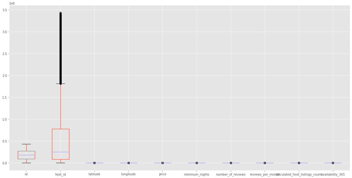

Records with outliers

q1 = rentals.quantile(.25)
q3 = rentals.quantile(.75)
iqr = q3 - q1
outliers_df = rentals[
    ((rentals < (q1 - 1.5*iqr)) | (rentals > (q3 + 1.5*iqr))).any(axis=1)
]
outliers_df.shape

(8544, 14)

There are Over 8500 outliers in the dataset

outliers_df.sample(5)

	id	host_id	host_name	neighbourhood	latitude	longitude	room_type	price	minimum_nights	number_of_reviews	last_review	reviews_per_month	calculated_host_listings_count	availability_365
12117	22620913	2888051	Lokke	Noord-West	52.41524	4.89218	Entire home/apt	80	4	2	2018-05-06	0.08	1	0
3511	7166128	16634603	Hermen	Centrum-Oost	52.36991	4.92621	Entire home/apt	110	5	7	2018-08-19	0.12	1	0
15707	32722735	246045083	Babette	De Baarsjes - Oud-West	52.36514	4.86184	Entire home/apt	120	2	8	2019-06-29	0.64	1	0
13425	26037649	193680275	Merle	Westerpark	52.38374	4.87314	Entire home/apt	125	5	5	2018-11-18	0.24	1	0
730	1277443	6952882	Jason & Lotte	Bos en Lommer	52.38129	4.85746	Entire home/apt	98	5	4	2014-07-07	0.06	1	0

Let’s check the percentage of outliers to the original dataset

print(f"Percentage of outliers: {outliers_df.shape[0]/rentals.shape[0]*100:.2f}")

Percentage of outliers: 50.04

It would be tricky to drop the records with outliers since that will reduce our dataset by half so we will leave them there. However, we will drop the host_id variable later on, right before modeling.

3. Data Analysis

3.1 Univariate Data Analysis

Top 10 Most common hosts

plt.figure(figsize=(20,12))
rentals.host_name.value_counts()[:10].plot(kind='bar')
plt.title("Top 10 Hosts")
plt.xlabel("Host Name")
plt.ylabel("Number of Listings")
plt.show()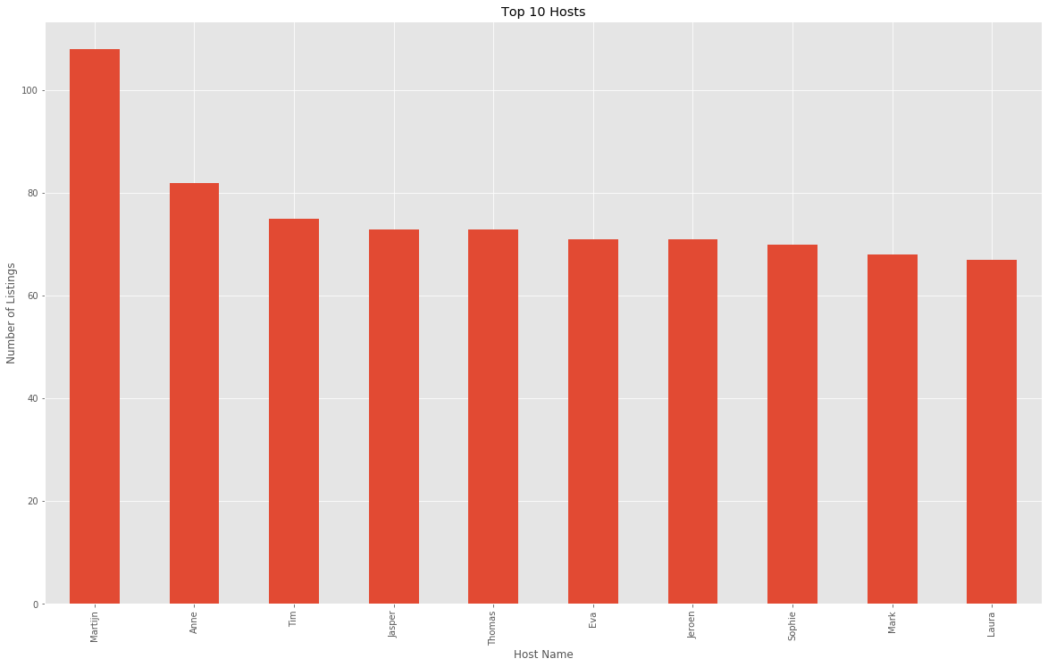

Martijn is the host name with most listings in the Airbnb rentals listing.

the top 10 most common neighbourhoods

plt.figure(figsize = (20, 12))
rentals.neighbourhood.value_counts()[:10].sort_values().plot(kind = 'barh')
plt.xticks(ha = "right")
plt.title("Top 10 Neighbourhoods")
plt.xlabel("Number of Listings")
plt.ylabel("Neighbourhood")
plt.show()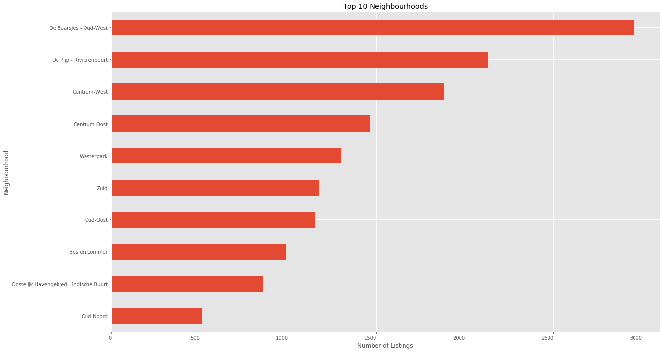

De Baarsjes - Oud-West Had the most number of rental listings

the most common room types

rentals.room_type.value_counts()

Entire home/apt    13308
Private room        3497
Hotel room           232
Shared room           38
Name: room_type, dtype: int64

plt.figure(figsize=(8,8))
rentals.room_type.value_counts().plot(kind='pie', autopct="%0.1f%%", labels=rentals.room_type.value_counts().index)
plt.legend()
plt.title("the most common room types")
plt.show()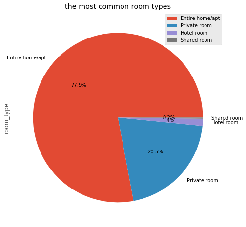

distribution of price

plt.figure(figsize = (14,8))
sns.distplot(rentals.price)
plt.title("Distribution of $price$")
plt.show()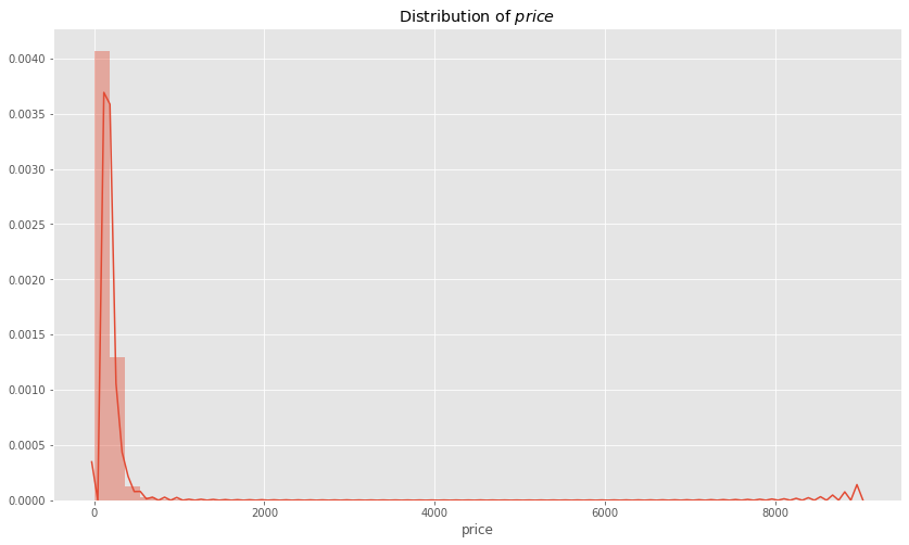

The distribution of price is skewed to the right and is not continous.

the top 10 most common minimum number of nights to spend

plt.figure(figsize=(20,10))
rentals.minimum_nights.value_counts()[:10].sort_values().plot(kind='barh')
plt.title("the top 10 most common minimum number of nights to spend")
plt.xlabel("Number of listings")
plt.ylabel("Minimum Nights")
plt.show()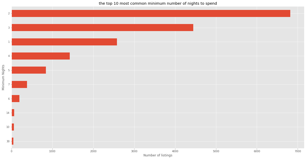

The most common minimum number of nights to spend is 2.

3.2 Bivariate Analysis

price by room type

rentals.hist('price', by='room_type', figsize=(20,12))
plt.show()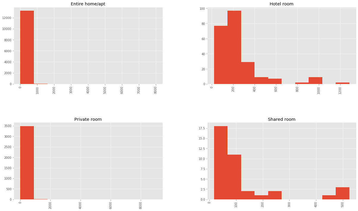

average price by neighbourhood

rentals.groupby('neighbourhood')['price'].mean().sort_values(ascending=False)

neighbourhood
Centrum-West                              203.653397
Centrum-Oost                              190.534247
Zuid                                      178.813243
Oud-Noord                                 168.763566
De Pijp - Rivierenbuurt                   166.601787
IJburg - Zeeburgereiland                  157.723077
Westerpark                                151.241140
De Baarsjes - Oud-West                    149.376228
Oud-Oost                                  144.606957
Watergraafsmeer                           141.199125
Buitenveldert - Zuidas                    137.690355
Oostelijk Havengebied - Indische Buurt    135.101163
Noord-Oost                                130.495833
Noord-West                                126.318885
Bos en Lommer                             122.525304
De Aker - Nieuw Sloten                    121.268908
Slotervaart                               119.791549
Geuzenveld - Slotermeer                   113.937143
Osdorp                                    103.418182
Gaasperdam - Driemond                      96.317757
Bijlmer-Centrum                            91.434343
Bijlmer-Oost                               89.696629
Name: price, dtype: float64

plt.figure(figsize=(20, 10))
rentals.groupby('neighbourhood')['price'].mean().sort_values(ascending=False)[:10].sort_values().plot(kind='barh')
plt.xlabel("Average Neighbourhood Price")
plt.title("average price by neighbourhood")
plt.show()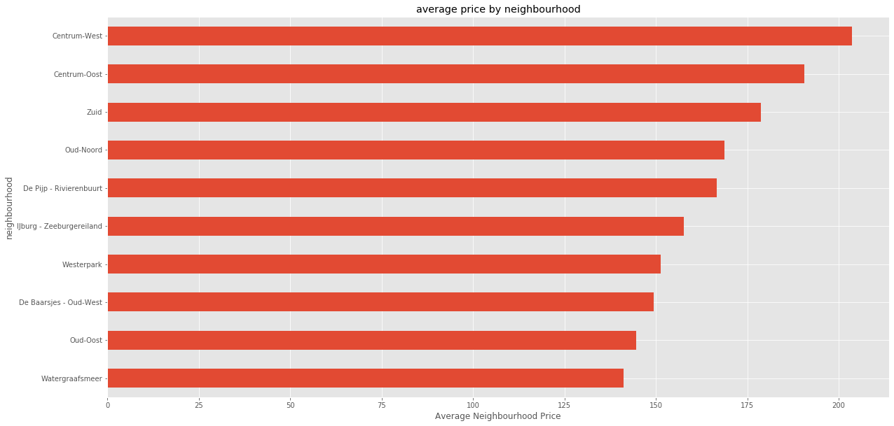

Based on neighbour hood, Centrum West Has the highest average weight of listings.

average price by minimum_nights

rentals.groupby('minimum_nights')['price'].mean().sort_values(ascending=False)[:15]

minimum_nights
365     3000.000000
200      999.000000
99       999.000000
52       429.000000
30       331.551020
222      300.000000
27       275.000000
48       250.000000
31       243.750000
150      203.000000
21       201.761905
15       197.888889
1000     185.000000
240      180.000000
28       175.900000
Name: price, dtype: float64

plt.figure(figsize=(20, 10))
rentals.groupby('minimum_nights')['price'].mean().sort_values(ascending=False)[:10].sort_values().plot(kind='barh')
plt.xlabel("Average minimum nights Price")
plt.title("average price by minimum nights")
plt.show()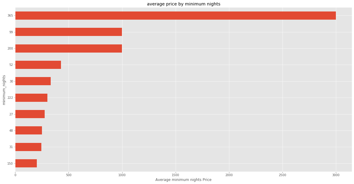

By average, those who spend 365 nights spend most price

3.3 Feature Engineering

rentals.head()

	id	host_id	host_name	neighbourhood	latitude	longitude	room_type	price	minimum_nights	number_of_reviews	last_review	reviews_per_month	calculated_host_listings_count	availability_365
0	2818	3159	Daniel	Oostelijk Havengebied - Indische Buurt	52.36575	4.94142	Private room	59	3	278	2020-02-14	2.06	1	169
1	20168	59484	Alexander	Centrum-Oost	52.36509	4.89354	Private room	100	1	340	2020-04-09	2.76	2	106
2	25428	56142	Joan	Centrum-West	52.37297	4.88339	Entire home/apt	125	14	5	2020-02-09	0.18	1	132
3	27886	97647	Flip	Centrum-West	52.38761	4.89188	Private room	155	2	217	2020-03-02	2.15	1	172
4	28871	124245	Edwin	Centrum-West	52.36719	4.89092	Private room	75	2	332	2020-03-16	2.82	3	210

rentals['room_type_encoded'] = LabelEncoder().fit_transform(rentals.room_type)
rentals.head()

	id	host_id	host_name	neighbourhood	latitude	longitude	room_type	price	minimum_nights	number_of_reviews	last_review	reviews_per_month	calculated_host_listings_count	availability_365	room_type_encoded
0	2818	3159	Daniel	Oostelijk Havengebied - Indische Buurt	52.36575	4.94142	Private room	59	3	278	2020-02-14	2.06	1	169	2
1	20168	59484	Alexander	Centrum-Oost	52.36509	4.89354	Private room	100	1	340	2020-04-09	2.76	2	106	2
2	25428	56142	Joan	Centrum-West	52.37297	4.88339	Entire home/apt	125	14	5	2020-02-09	0.18	1	132	0
3	27886	97647	Flip	Centrum-West	52.38761	4.89188	Private room	155	2	217	2020-03-02	2.15	1	172	2
4	28871	124245	Edwin	Centrum-West	52.36719	4.89092	Private room	75	2	332	2020-03-16	2.82	3	210	2

rentals.neighbourhood.nunique()

22

rentals_2 = rentals.drop(columns=['id', 'host_id', 'host_name', 'neighbourhood', 'last_review', 'room_type'])
rentals_2.head()

	latitude	longitude	price	minimum_nights	number_of_reviews	reviews_per_month	calculated_host_listings_count	availability_365	room_type_encoded
0	52.36575	4.94142	59	3	278	2.06	1	169	2
1	52.36509	4.89354	100	1	340	2.76	2	106	2
2	52.37297	4.88339	125	14	5	0.18	1	132	0
3	52.38761	4.89188	155	2	217	2.15	1	172	2
4	52.36719	4.89092	75	2	332	2.82	3	210	2

4. Data Modeling

X = rentals_2.drop(columns=['price'])
y = rentals_2.price

X = StandardScaler().fit_transform(X)
X[:5]

array([[ 0.01659773,  1.45384638, -0.02542703,  4.36034888,  0.92231486,
        -0.21630069,  1.18401885,  1.92103452],
       [-0.02390588,  0.11006752, -0.15344314,  5.44467417,  1.44564814,
         0.06606432,  0.54605829,  1.92103452],
       [ 0.45968261, -0.17479788,  0.67866153, -0.4141802 , -0.4832088 ,
        -0.21630069,  0.8093436 , -0.52593784],
       [ 1.3581262 ,  0.0634787 , -0.08943509,  3.29351271,  0.98960057,
        -0.21630069,  1.21439792,  1.92103452],
       [ 0.10496923,  0.03653577, -0.08943509,  5.30476123,  1.49050528,
         0.34842932,  1.59919952,  1.92103452]])

X_train, X_test, y_train, y_test = train_test_split(X, y, test_size=.3)

For purposes of simplicity, we will work with the following regressors:

• Decision Tree Regressor
• Random Forest Regressor

4.1 Normal Modeling

dt = DecisionTreeRegressor()
rf = RandomForestRegressor()

dt.fit(X_train, y_train)
dt_pred = dt.predict(X_test)
print(f"DT RMSE: {np.sqrt(mean_squared_error(y_test, dt_pred)):.2f}")
print(f"DT R2: {r2_score(y_test, dt_pred):.2f}")

DT RMSE: 249.36
DT R2: -5.03

rf.fit(X_train, y_train)
rf_pred = rf.predict(X_test)
print(f"rf RMSE: {np.sqrt(mean_squared_error(y_test, rf_pred)):.2f}")
print(f"rf R2: {r2_score(y_test, rf_pred):.2f}")

rf RMSE: 111.97
rf R2: -0.22

y.sample(int(y.shape[0]*.1)).mean()

154.93731693028704

Both models are performing well, we will use Random Forest Regressor because it is the best perfroming model producing the best fit.

4.2 Modeling with Grid Search

rf.get_params()

{'bootstrap': True,
 'ccp_alpha': 0.0,
 'criterion': 'mse',
 'max_depth': None,
 'max_features': 'auto',
 'max_leaf_nodes': None,
 'max_samples': None,
 'min_impurity_decrease': 0.0,
 'min_impurity_split': None,
 'min_samples_leaf': 1,
 'min_samples_split': 2,
 'min_weight_fraction_leaf': 0.0,
 'n_estimators': 100,
 'n_jobs': None,
 'oob_score': False,
 'random_state': None,
 'verbose': 0,
 'warm_start': False}

param_grid = {
    'bootstrap': [True, False],
    'n_estimators': [100,110,120,130,140],
    'max_depth': [10, 20, 30, 40, 50]
}
grid_search = GridSearchCV(rf, param_grid=param_grid, cv=5, n_jobs=-1)
grid_result = grid_search.fit(X_train, y_train)
print(f"Best Score: {grid_result.best_score_}\nBest Parameters: {grid_result.best_params_}")

Best Score: -0.060206490328136075
Best Parameters: {'bootstrap': True, 'max_depth': 40, 'n_estimators': 140}

We will use the generated parameters to train our model

rf_gs = RandomForestRegressor(bootstrap=True, max_depth=40, n_estimators=140, n_jobs=-1)
rf_gs.fit(X_train, y_train)
rf_gs_pred = rf_gs.predict(X_test)
print(f"RMSE: {np.sqrt(mean_squared_error(y_test, rf_gs_pred)):.2f}\nR2 Score: {r2_score(y_test, rf_gs_pred):2f}")

RMSE: 112.40
R2 Score: -0.225879

4.3 Modeling with Random Search

random_search = RandomizedSearchCV(rf, param_distributions=param_grid, cv=5)
random_result = random_search.fit(X_train, y_train)
print(f"Best Score: {random_result.best_score_}\nBest Parameters: {random_result.best_params_}")

Best Score: -0.11714015166923782
Best Parameters: {'n_estimators': 120, 'max_depth': 40, 'bootstrap': True}

rf_rs = RandomForestRegressor(bootstrap=True, max_depth=40, n_estimators=140, n_jobs=-1)
rf_rs.fit(X_train, y_train)
rf_rs_pred = rf_rs.predict(X_test)
print(f"RMSE: {np.sqrt(mean_squared_error(y_test, rf_rs_pred)):.2f}\nR2 Score: {r2_score(y_test, rf_rs_pred):2f}")

RMSE: 108.37
R2 Score: -0.139507

4.4 Modeling with Bayesian Optimization

def objective(space):
    model = RandomForestRegressor(
        n_estimators=space['n_estimators'], 
        bootstrap=space['bootstrap'], 
        max_depth=space['max_depth']
    )
    accuracy = cross_val_score(model, X_train, y_train, cv=5).mean()
    return {'loss': -accuracy, 'status': STATUS_OK }
param_grid = {
    'bootstrap': hp.choice('bootstrap',  [True, False]),
    'n_estimators': hp.choice('n_estimators', [100,110,120,130,140]),
    'max_depth': hp.quniform('max_depth', 10, 50, 10)
}
trials = Trials()
best = fmin(fn= objective,
            space= param_grid,
            algo= tpe.suggest,
            max_evals = 100,
            trials= trials)
best

100%|███████████████████████████████████████████| 100/100 [1:20:39<00:00, 48.39s/trial, best loss: 0.05966699243049871]

{'bootstrap': 0, 'max_depth': 10.0, 'n_estimators': 3}

btsp = {0:True, 1:False}
n_est = {0:100,1:110,2:120,3:130,4:140}
rf_bo = RandomForestRegressor(
    bootstrap=btsp[best['bootstrap']],
    max_depth = best['max_depth'],
    n_estimators=n_est[best['n_estimators']]
).fit(X_train, y_train)
rf_bo_pred = rf_bo.predict(X_test)
print(f"RMSE: {np.sqrt(mean_squared_error(y_test, rf_bo_pred)):.2f}\nR2 Score: {r2_score(y_test, rf_bo_pred):2f}")

RMSE: 107.42
R2 Score: -0.119587

5. Summary of Findings

• By performing hyperparameter tuning, we have achieved a model that achieves optimal predictions
• Compared to GridSearchCV and RandomizedSearchCV, Bayesian Optimization is a superior tuning approach that produces better results in less time.

6. Recommendations

• More data need to be added. When we have more data, the model will be more accurate and this will minimize bias in prediction.
• More features need to be added. In addition to the data we need more features about rental listings so that the data won’t depend on minimal features during prediction

7. Challenging the Solution

• The question was clear since we were required to perform hyperparameter tuning techniques to your most accurate model in an effort to achieve optimal predictions.
• This was a right data but Major imporvements need to be added to the data, more features need to be added to make the model more accurate. Missing values needs to be addressed during data collection
• To improve the solution, more data is needed to train the model to be as accurate as possible in the prediction.